Here is an exciting new announcement from Google on recent updates to features in Sheets, which can help users streamline processes and make working in Sheets even easier.
Google knows it can be time consuming to perform repetitive tasks like updating data in a spreadsheet. Additionally, maintaining the structure and format of the data can be difficult when there are multiple people updating the document.
To help solve this, they have announced Tables in Google Sheets. With Tables, you can simplify and accelerate spreadsheet building by bringing format and structure to unorganized ranges. By selecting your data range and going to Format > Convert to Table, Sheets now does the heavy lifting to format and organize data with a polished design including column types, filters, color coding, dropdown menus and more.
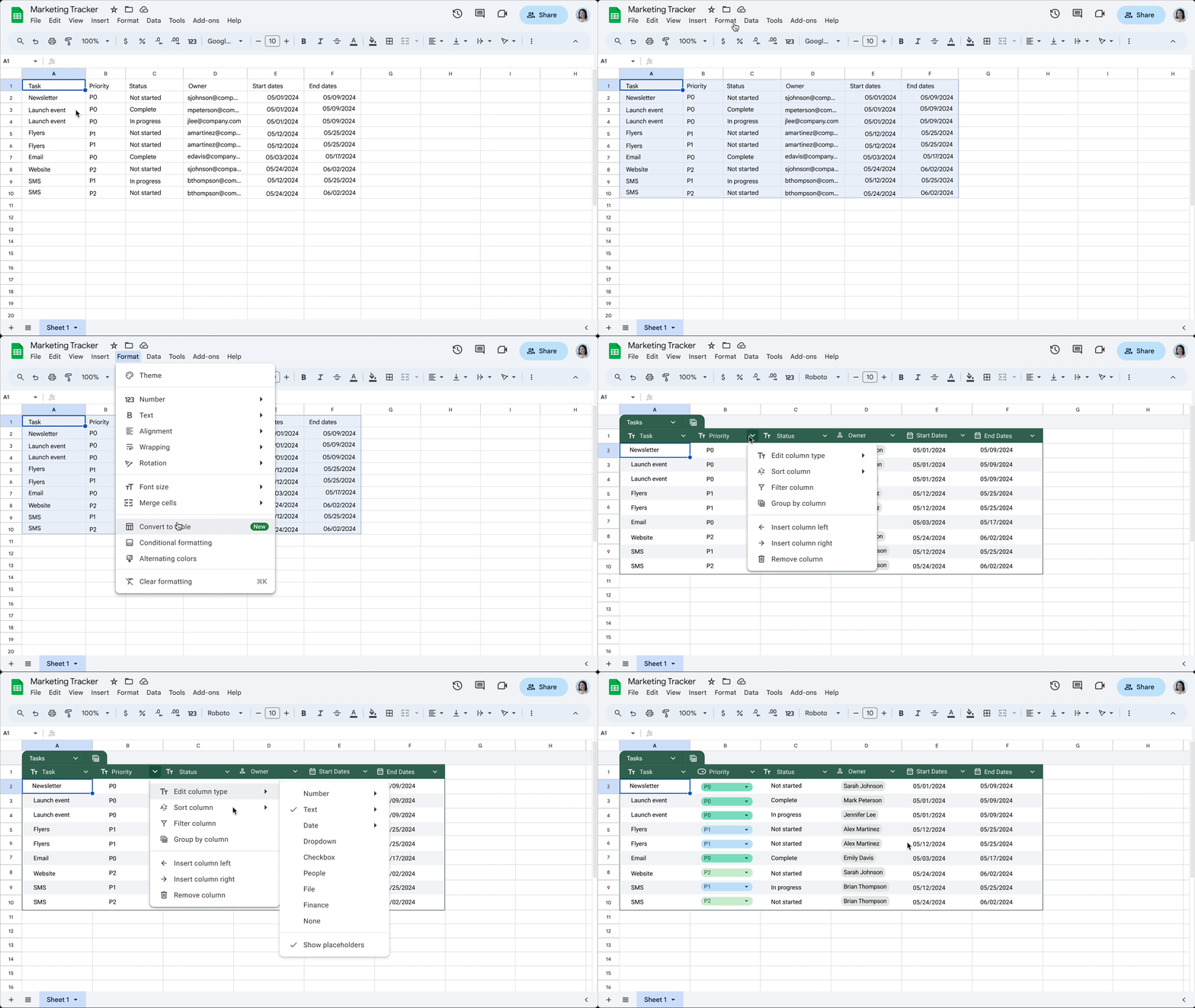
Here’s how using tables reduces the time you would usually spend manually formatting data:
- Auto-applied formatting: When you convert your data to a Table, Sheets automatically applies formatting to polish your data so that all inputs are properly aligned, reducing the need for manual changes. You can further customize your Table by changing colors, readjusting the row height, and more.
- Column types: For each column, you can set the appropriate column type (e.g., date, currency, dropdown), and your Table will make sure all entered data has the right formatting based on the column type. Data entered that does not align with a set column type will result in a warning.
- Unified menu: Above the Table, you will see a menu option to manage Table-level settings (e.g., adjust table range) and take action (e.g., create a filter view for your Table).
- Table references: Table references are a special way to refer to a Table or parts of a Table in a formula. When you convert your data to a Table, Sheets provides a name for the Table and each column header. When you reference Table elements by name, the references update whenever you add or remove data from the Table. For example: Instead of explicit cell references: =COUNTIF(B2:B10, “P0”), you can use Table references: =COUNTIF(Task_tracker[Priority], “P0”).
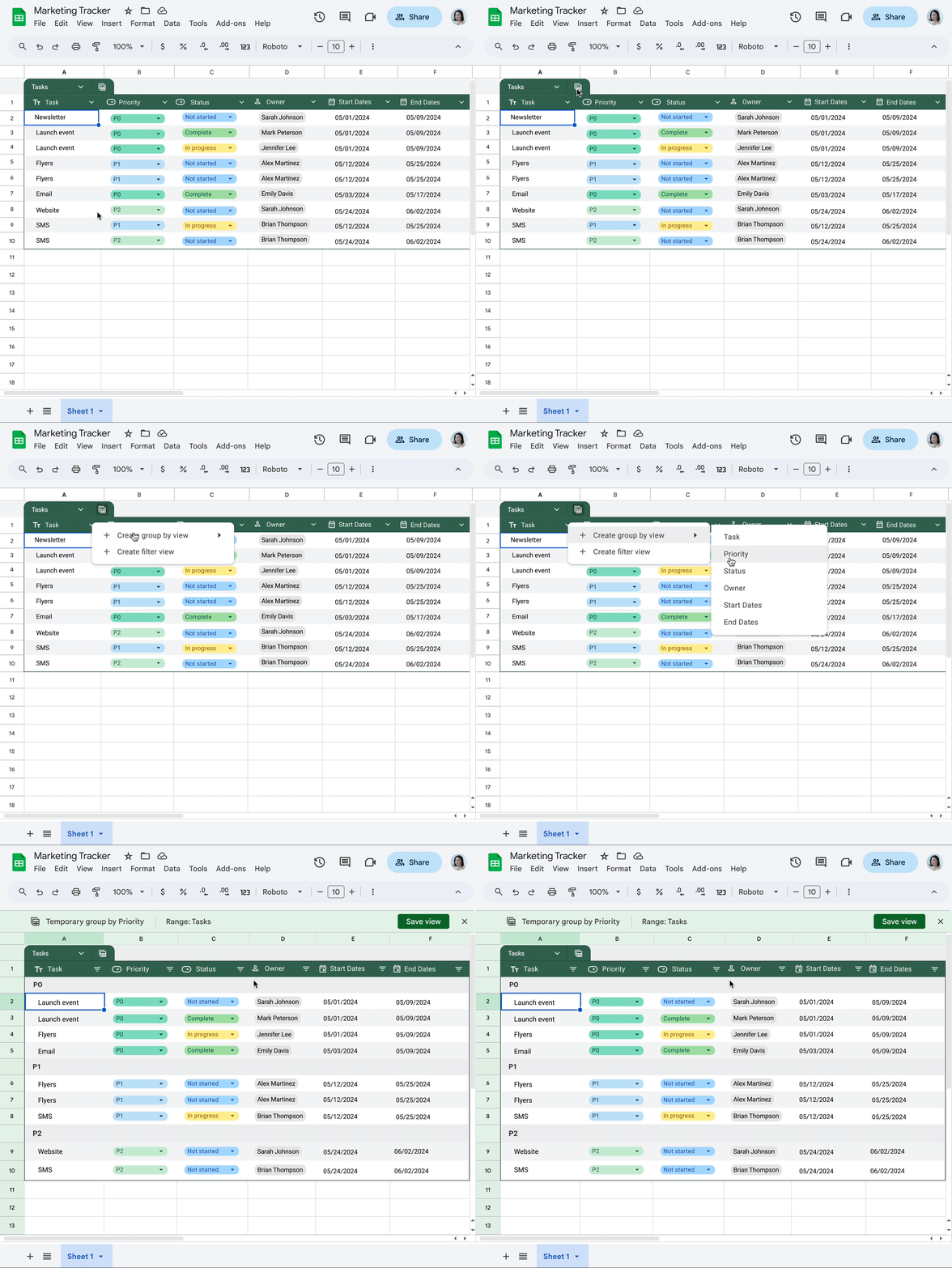
When you are using Tables, you’ll also have access to our new type of view, group by, where you can aggregate your data into groups based on a selected column. For instance, you can decide to group all data at the same priority level in one place, as shown below.
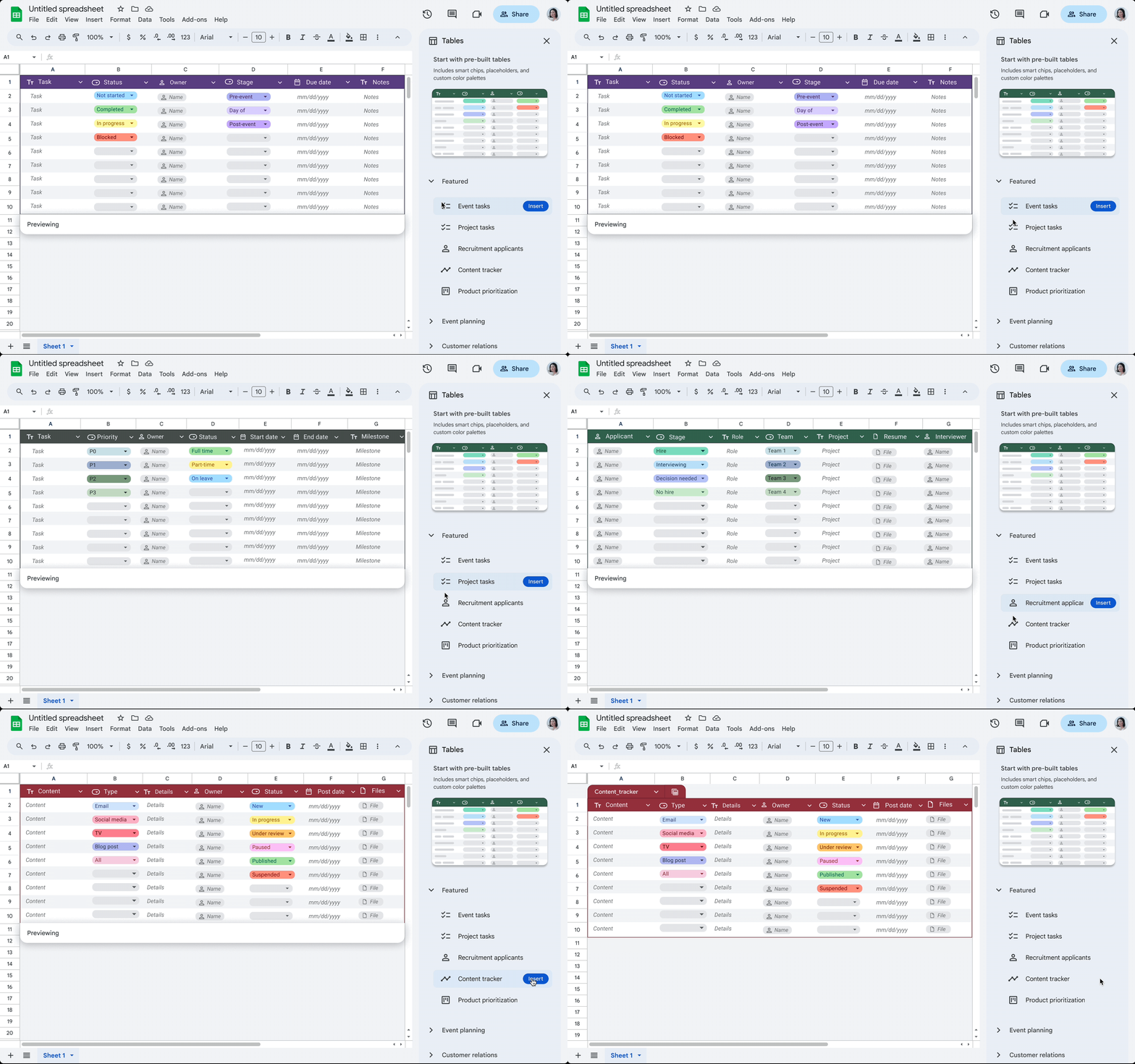
They’re also introducing pre-built Tables that you can populate with common data types for everyday tasks like project management, inventory management, event planning and more. Now with pre-built Tables, you never have to build a spreadsheet from scratch again.
Tables is available to all Workspace users now with rapid release, and it will begin rolling out generally by June 6.

